 Matlab s-functions seem scarier than they really are. Understanding how Simulink works and what goes behind the scenes when you simulate helps learning s-functions. In this blog I’ll show you how to write a simple s-function to generate variable width pulse train (variable width PWM or variable duty-cycle pulse generator). One often requires that pulse width (or duty cycle) of a pulse generator be variable via a signal rather than specified as a constant in block parameters. s-function demos has an example to the same effect, but I have simplified it quite a bit to avoid confusion to beginners from unnecessary methods and stuff (like Dwork).
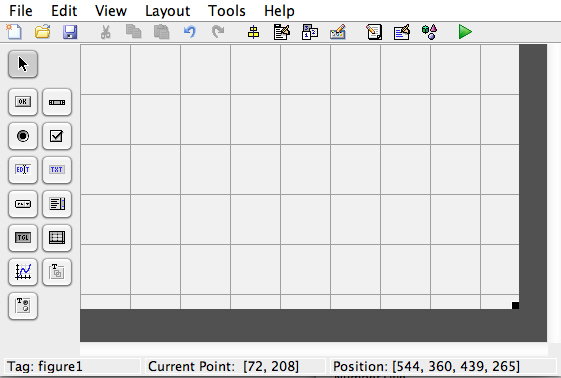
Start with a new model file with pulse generator block, a level-2 s-function block and a repeating sequence block. We shall use the repeating sequence to generate a triangular wave and feed it to the s-function block which will change pulse width of the pulse generator block according to the instantaneous value of the triangular wave.
An s-function block has two block parameters – the name of the s-function and the parameters you want to pass into the s-function. You can right away name your s-function and click ‘edit’ and Matlab will create a new file (if a file with that name doesn’t exist ). Alternatively, you can open a blank new m-file and use it to define the s-function. Define the primary function with no outputs, but with one input, say ‘block’. Inside there you just need to call setup(block), which is going to be another function we need to define in the same file.
function variablePulseWidth(block)

% Variable Pulse Width s-Function

% Use this block to vary pulse width (duty-cycle) of a pulse generator

% Connect the input port to the signal which dictates the duty cycle as a

% percentage. Range of values the signal can take would be 0 to 100 (both

% end points excluded).

% (c) Planck Technical,2013

setup(block)
Writing the s-function begins with defining the setup method. Setup initialises the s-function block by setting some basic attributes like number of input & output ports, their types and sizes, number of parameters the s-function should accept from the block-parameters window, sample time of the block, etc. Here, you will also need to declare other callback methods that you will be using to design the functioning of the block. Predominantly many of these methods have only one input argument, which, we will call ‘block’ (- its a special datatype of class Simulink.MSFcnRunTimeBlock).
function setup(block)

% Register number of ports

block.NumInputPorts = 1;

block.NumOutputPorts = 0;
We do not need any output ports for this s-function as the output will be from the pulse generator and we will only be using this s-function to change the pulse width setting of the generator block. Next, properties of each of these input and output ports have to be specified.
 % Specify inport properties

block.InputPort(1).Dimensions = 1;

block.InputPort(1).DatatypeID = 0; % double

block.InputPort(1).Complexity = 'Real';

block.InputPort(1).DirectFeedthrough = false;

%

% No output port, So no properties to set here
With a little foresight, its recommended that we use s-function dialog box parameters to specify name of the pulse generator block whose pulse width has to be varied. This is handy if there are multiple pulse blocks and each of them needs to be controlled, may be with different signal.
 % We'll use Pulse Generator block name as input to s-function

block.NumDialogPrms = 1;
Specify the sample time of the block as a vector of two values [sampling period, offset]. Here, the sample time is set to be inherited.
% Register sample time to inherited

block.SampleTimes = [-1 0];
After initialising the block using above lines of code, Simulink likes to get on with the business of computing the block outputs. However, before that there could be additional things a user might be interested in doing before computing the outputs. Things like some initialisation tasks or computations associated with this (or other) block(s). For such things, Simulink provides methods like Start and InitializeConditions. There might also be some tasks which are to be carried out only at major time steps, or at termination of simulation which can be addressed using one or more of methods listed here. Of all these methods, only two – ‘Outputs’ and ‘Terminate’ are required to be declared while the rest are optional. In our example, there isn’t really a need for these, so the code below only shows the two necessary methods.
% Register all methods to be used in this file

block.RegBlockMethod('Outputs', @outputs); % Required

block.RegBlockMethod('Terminate', @terminate); % Required
During Simulation, ‘Outputs’ method is called at each time step (major and minor). ‘Start’ & ‘InitializeConditions’ are called at the beginning of the simulation. ’Terminate’ is called only after simulation (or its termination) or when an s-function block is deleted. Declaring all methods to be used in the file marks end of the ‘setup’ method. All these registered methods now need to be defined.
Our plan is to utilise ‘Outputs’ method, which is executed at every time step, to change the pulse width parameter of the Pulse block.
function outputs(block)

pulseBlock = block.DialogPrm(1).Data;

pulseBlockPath = [get_param(block.BlockHandle,'parent'),'/',pulseBlock];

set_param(pulseBlockPath,'PulseWidth',num2str((block.InputPort(1).data)));
The first line fetches the dialog parameter from the block parameters dialog box, where user mentions of the name of the Pulse block. E.g. if user mentions ‘Pulse Generator 1′ in the dialog box, the same string is fetched into the variable ‘pulseBlock’. If user declares two parameters in the setup method, the dialog box can input two input arguments and the second one can be accessed as block.DialogPrm(2).Data. The second line makes the full path to the pulse block, which is used in third line to set ‘PulseWidth’ parameter of this block. Data coming into the input port of the s-function is accessed as block.InputPort(1).data. If there are two input ports declared in setup method, the data into second port can be accessed as block.InputPort(2).Data. Whenever block parameters are being set, they need to be written as strings. Hence, numeric data in the input port of s-function is converted to string using num2str.
We will not use terminate method, it may be safely left blank.
function terminate(block)
Save the m-file with a filename exactly matching the function name used at the very top. You are now good to start using the variablePulseWidth s-function.

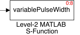
Variable Pulse Width Pulse Generator with s-function
Its possible that you get an error complaining that PulseWidth must be a number between 0 and 100. That happens at the beginning of simulation when the s-function block is executed before the block feeding1 its input, i.e. the Repeating Sequence source block. If Simulink executes s-function before its feeding block in, there will be no data present at its input port, i.e., block.InputPort(1).data is zero. However, zero is invalid entry for pulse width. This issue can be addressed by changing the block execution order of these two blocks. Right-click a block to choose ”Properties” and enter a number (integers starting with zero) in ‘Priority’ field. Entering a greater integer for s-function compared to that of its feeding block lowers the priority of the s-function block and updating the figure (CTRL+D) will show you new block execution order (if you have it enabled from Display Tab > Blocks > Block Execution Order).
The initial value chosen for pulse width can be either specified manually in the block parameters window of Pulse Generator block. Or, it can be done via s-function’s optional method Start or InitializeConditions. E.g. I can include one of these methods in the file (after registering it in setup method as block.RegBlockMethod(‘InitializeConditions’, @initConditions) ). The function name you choose can be anything- it doesn’t have to match the method name.
function initConditions(block)

pulseBlock = block.DialogPrm(1).Data;

pulseBlockPath = [get_param(block.BlockHandle,'parent'),'/',pulseBlock];

set_param(pulseBlockPath,'PulseWidth','50');
The above function would ensure the first pulse will be of 50% duty cycle. Instead of hard coding it inside the function, this can be made a user specifiable parameter in the s-function dialog box. Then, your s-function will have 2 parameters and you will specify them separated by commas in the parameters box as ‘Pulse Generator 1′,50. Note that the name of block must be in single quotes as its a string. The parameter 50 can be specified as a number or as a string ’50′, but must be used accordingly in the InitializeConditions function.
The built-in s-function templates make writing s-functions a bit easier. Matlab provides two templates – a basic one (msfcntmpl_basic.m) and a full template (msfcntmpl.m). The former lists 7 most used (of the 25 available) callback methods, while the latter lists almost all. To open these templates, click on the link in documentation or use these links
>> edit([matlabroot,'/toolbox/simulink/blocks/msfuntmpl_basic.m'])

>> edit([matlabroot,'/toolbox/simulink/blocks/msfuntmpl.m'])
In a followup post someday, I’ll try and highlight more advanced uses of s-functions, using these other optional methods that I skipped here. How have your experiences been with s-functions? Do you like to see a specific use of s-functions in a followup blog post here? Share your thoughts and comments.
EDIT: Model file attached as requested by a commenter: varpulsewidthexample All the code is in the post, just use it in a file named varpulsewidexample.mdl